# Dr. M. Baron, Statistical Machine Learning class, STAT-427/627

# REGRESSION DIAGNOSTICS

# Let's change the folder to the one where we have data

> setwd("C:\Users\baron\627\data")

> load("Auto.rda")

> names(Auto)

[1] "mpg" "cylinders" "displacement"

[4] "horsepower" "weight" "acceleration"

[7] "year" "origin" "name"

> attach(Auto)

> reg=lm(mpg ~ year + acceleration + horsepower + weight)

> par(mfrow=c(2,2))

> plot(reg)

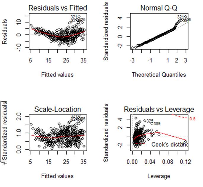
# STUDENTIZED RESIDUALS AND OUTLIERS

> t = rstudent(reg)

> plot(t)

> t[ abs(t) > 3 ]

243 321 324 325 328 382

3.338459 4.272284 3.446234 3.651403 3.236226 3.024362

# Which of these residuals can be considered as outliers?

# Compare with the Bonferroni-adjusted quantile from t-distribution.

> qt( 0.05/2/392, 387 )

[1] -3.870293

> t[ abs(t) > abs(qt( 0.05/392/2, 387 )) ]

321

4.272284

# Testing NORMALITY

> shapiro.test(t)

Shapiro-Wilk normality test

data: t

W = 0.97109, p-value = 5.101e-07

# Also look at the Normal Q-Q plot above. Shapiro-Wilk statistic W measures how close the graph is to a straight line.

# Testing HOMOSCEDASTICITY (constant variance). This is the Breausch-Pagan test.

> ncvTest(reg)

Non-constant Variance Score Test

Variance formula: ~ fitted.values

Chisquare = 22.04621 Df = 1 p = 2.66165e-06

# INFLUENTIAL DATA

> infl = influence(reg)

# Gives hat diagonals H_ii, the vector of coefficients (without the ith case), s = RMSE (without the ith case)

> leverage = infl$hat

> plot(leverage)

> 5/length(mpg)

[1] 0.0127551

> summary(infl$hat)

Min. 1st Qu. Median Mean 3rd Qu. Max.

0.002781 0.007543 0.010640 0.012760 0.014740 0.120500

> leverage[ leverage > 0.03 ]

> infl$coefficients

> infl$sigma

# ADDITIONAL PACKAGE "CAR" (Go to "Packages" tab and choose "car")

> library(car)

> outlierTest(reg)

rstudent unadjusted p-value Bonferonni p

321 4.272284 2.4397e-05 0.0095635

> cook = cooks.distance(reg)

> plot(cook)

# The Cook’s distance measures the effect of deleting the i-th observation

> influence.measures(reg)

# Besides the Cook’s distance, it calculates DFBETS, DFFITS, and other measures of influence

# VARIANCE INFLATION FACTORS

> vif(reg)

year acceleration horsepower weight

1.228910 2.519844 8.813443 5.303347